Quantcast
Channel: Diffusion Imaging; Introduction, tutorials and background on diffusion tensor imaging and techniques
Viewing all 30 articles
Browse latest View live

DTI Quality Control - Part 4: Further reading

$
0
0


Analysis of diffusion images are complicated by the fact that errors can be easily hidden inside the calculated tensor data and not clearly show up in your final processed FA image. Quality control is thus an essential step to ensure data quality. Three previous blog post were dedicated to quality control after acquisition, during tensor calculation and suggested tools to help with QCThis post will suggest some articles for further reading, mainly focussed on best practice during quality control. 

To start off I would like to suggest this excellent article by Tournier, Mori and Leemans. In this publication the authors discuss a number of issues that you can pay attention to. Like the examples from figure 1 in their article. There are more examples in their full article that you can check out. 

You might also like the aptly named hitchhiker's guide to diffusion tensor imaging - previously discussed in this post. They give a clear overview of steps important for effective diffusion imaging processing and quality control:


An other previously discussed (on the diffusion imaging Facebook page, check it out!) article is written by Derek Jones et al. and discusses the do's and don'ts of diffusion MRI. Less involved with practical quality control tips, and thus more involved with global expectation  management and best use practices:
" In order to encourage the use of improved DW-MRI methods, which have a better chance of characterizing the actual fiber structure of white matter, and to warn against the misuse and misinterpretation of DTI, we review the physics of DW-MRI, indicate currently preferred methodology, and explain the limits of interpretation of its results. We conclude with a list of ‘Do's and Don'ts’ which define good practice in this expanding area of imaging neuroscience."

A recent paper by a german neurosurgery group gives a comprehensive overview of software packages that can be used for fiber tracking and compares their efficacy running different fiber tracking algorithms. Results are reviewed by a physicist, neuroradiologist and neurosurgeon (lower scores are better):

It is clearly not easy to acquire diffusion images without error, the successful acquisition of diffusion imaging data in neonates is a factor more complicated. This article give some important tips for acquisition guidelines - for example note that gray/white matter contrast is not nearly as pronounced yet, and sometimes looks opposite in brightness as compared to older populations. This is due to reduced myelination of the white matter at this stage, and can be countered by changing the relaxation time of the T1 or T2 scan. They also go into details of effective quality assessment, to catch issues arising due to movement, pulsation or reduced head size.

Finally, a group at Vanderbilt suggest a number of complementary metrics that can be used for quality assurance and compare their unified pipeline with visual inspection and show that their method can produce a 70% time saving. More information on their methods in their article.
Thanks to Andy Alexander at the Waisman Center for brain imaging and behavior for his database on QC articles.

From diffusion weighted images to the diffusion tensor model: a simplified case example

$
0
0


A guest post by Rodrigo Dennis Perea on the computational models for estimating the diffusion tensor from diffusion weighted images: 
"When I first started working with DTI, I had a hard time understanding the derivation of the diffusion tensor from what was acquired on the scanner, the diffusion weighted image (DWI). Once I understood this process a little better I decided to create a brief review. I hope this will help you! It might be lacking information or it might be too implicit so please feel free to ask me anything if you need more detailed information."
                                                                                               
I have to thank Peter B. Kingsley for his very helpful publication on this topic: http://onlinelibrary.wiley.com/doi/10.1002/cmr.a.20048/abstract 
First, it is worth noting that this example will highlight the computations in a single voxel (e.g. x=76, y=64, z=21). Essentially, a similar approach will be applied to every voxel in the entire MRI scan. The figure below illustrates our example where we have six DWI's, and the sample voxel is denoted by a small color coded square: 

The simplified diffusion matrix will look like this:
Which will translate into this tensor:

Next the Stejskal-Tanner equation is of importance, this equation shows how there will be a reduction in the signal due to the application of a pulse gradient, this change will be proportional to the amount of diffusion: 

Image[1] 
It is important to notice that we will solve for tensor D given the other parameters from the MRI acquisition. Sk is the intensity at the "single voxel" when a specific gk gradient direction is applied (e.g. a 1x3 vector for the x,y,z direction).  b0 is the no diffusion signal and S0 is the intensity value you get from the no-diffusion signal. So lets begin...
A random MRI-DWI sequence (lets say sample_001) is used as an example. Given the following gradient vectors with their specific intensity values at an specific voxel location in the brain, we will derive equation [1]  to solve for the simplest case with only 7 volumes (1 3D volume with no diffusion and 6 3D volumes with pulse gradient directions).
A simple approach: The “H” approach: Six gradient directions (Sk) images “plus” a no-diffusion image (S0)
Given the following gradient direction pulses and intensities with a b-value of 800 s/mm2:
          
Given equation Stejskal-Tanner equation:
Image[1] 
with gk­:
Image [2]                 
And D:
Image    [3]
We can solve expand equation [1] in terms of D:
Image  [4]
Where the subscript “i” denotes each gradient direction pulse ("i" in this case will go from 1 to 6).  One approach to solve this system of equation is to use matrix algebra. Thus let express D as a six-element column vector, d:
Image      [5]
With a six-element row matrix containing a large M x 6 matrix, where M is the number of gradient directions (in this case M=6):
H_6[6]
Lastly, let’s define a Y matrix for the left side of equation [4]:
Image[7]
Thus we can express equation [4] with the following 6 directions as:
Image    [8]
With exactly six directions, there is an exact analytic solution and can be solved using standard methods such as the Cramer’s rule:
Image   [9]
Using these equation, I was able to create functions in matlab. I also compared my accurate results with FSL dtifit, which gave me similar results. 
I'll be more than happy to share my matlab functions and explain these in more detailed if needed. 

Neuroscience Information Framework for DTI resources

$
0
0


The Neuroscience Information Framework (NIF) is an initiative by NIH blueprint to bring together all knowledge on neuroscience. Of course DTI is part of this. Find everything NIF put together on DTI here:

From their website (http://neuinfo.org/about/index.shtm): 

About NIF

The Neuroscience Information Framework is a dynamic inventory of Web-based neuroscience resources: data, materials, and tools accessible via any computer connected to the Internet. An initiative of the NIH Blueprint for Neuroscience Research, NIF advances neuroscience research by enabling discovery and access to public research data and tools worldwide through an open source, networked environment.

NIF OFFERS:
  1. search portal for researchers, students, or anyone looking for neuroscience information, tools, data or materials.
  2. Access to content normally not indexed by search engines, i.e, the "hidden web"
  3. Tools for resource providers to make resources more discoverable, e.g., ontologies, data federation tools vocabulary services
  4. Tools for promoting interoperability among databases
  5. Standards for data annotation
  6. The NIFSTD ontology covering the major domains of neuroscience, e.g., brain anatomy, cells, organisms, diseases, techniques
  7. Services for accessing the NIF vocabulary and NIF tools
  8. Best practices for creating discoverable and interoperable resources
  9. Data annotation services: NIF experts can enhance your resource through semantic tagging (contact us)
  10. NIF cards: Easy links to neuroscience information from any web browser (See examples)
  11. Ontology services: NIF knowledge engineers can help create or extend ontologies for neuroscience
The NIF project is designed to serve the biomedical research community. The more participation from the community, the better the NIF. We welcome all feedback and suggestions and are actively looking for resource providers to make their resources accessible through the NIF. We offer a variety of methods for making resources searchable through the NIF. For more information or to recommend a resource, follow the link to Register Your Resource, or send us an e-mail atcuration@neuinfo.org.
Collaborating institutions working on the current version of NIF include University of California, San Diego, California Institute of Technology, George Mason University, Yale University Medical College, and Washington University.

The History of NIF

Established in 2004, the NIH Blueprint for Neuroscience Research brings the 16 NIH Institutes, Centers and Offices that support neuroscience research into a collaborative framework to coordinate their ongoing efforts and to plan new cross-cutting initiatives. Working together, representatives from the partner Institutes, Centers, and Offices identify pervasive challenges in neuroscience and any technological barriers to solving them.
Early in their deliberations Blueprint representatives recognized that a framework for identifying, locating, relating, accessing, integrating, and analyzing information from the neuroscience research enterprise is critical to enhancing cooperative activities in the neurosciences. A Broad Agency Announcement was issued, and in 2005, the Blueprint began support for a new initiative known as the "Neuroscience Information Framework" (NIF).
The first phase of NIF was led by Dr. Dan Gardner at Weill Cornell Medical College. During this phase, the NIF produced awhite paper outlining the current state of neuroscience resources. The project also produced a registry of neuroscience-relevant resources, an extensive vocabulary for describing resources and their content, and an initial version of a concept-based query system that could be used to query across diverse types of resources. The current phase of NIF is led by Dr. Maryann Martone at UCSD. This phase is devoted to hardening and maintaining the NIF while continuing to expand its resources and increase its usability and functionality.

DTI processing with Brainvoyager

$
0
0


BrainVoyager QX is a powerful neuroimaging software package. It started as a tool for the analysis of anatomical and functional MRI data sets but has evolved over the years into a multi-modal analysis tool for fMRI, DTI, TMS, EEG and MEG data. The software is highly optimized and user friendly running on all major computer platforms including Windows (XP/Vista/7), Linux (i.e. Ubuntu, SUSE, Fedora) and Mac OS X (10.6 or higher).


Overview of DWI Analysis Steps in BrainVoyager

Single-run data in measurement space:


Single-run data in normalized 3D space:


Group comparison:


More information here:
http://support.brainvoyager.com/diffusion-weighted-imaging.html


Non-isotropic voxels; What to do and why

$
0
0


A recent question came up on the forum that was concerned with isotropic versus non-isotropic voxel sizes:

Hi, I am trying to process some DTI data using FSL for TBSS or Voxel based comparison. I am following the basic guideline from http://www.cabiatl.com/Resources/Course/tutorial/html/dti.html and this works good.

However, I found my DTI data set is not isotrophic, about 0.9 x 0.9 x 3 mm.
My question is

  1. Does the DTI voxel size matter for TBSS or VBM? Can I run those statistical using this asymmetric voxel data?
  2. If it matters, how can I overcome the problem? I have FSL on my macbook and Matlab.
  3. How about the effect of this asymmetric voxel for tractography?

My response:

That is a great question, I think it is indeed important to use isotropic voxels for DTI. You can run VBM and TBSS on non-isotropic voxels, interpolation will not likely alter your results, although isotropic acquisition might have.

It is a different story for tractography, where it will be important to interpolate to isotropic voxels. Non-isotropic voxels can negatively influence fiber tracking results, eg. you are less likely to find specific smaller/bendier tracts. My personal experience when running different tests, is that higher (isotropic) resolution (even when through interpolation) will improve tractography results. Although you'll have to keep an eye on your computing power, it is easy to "break" your processor/RAM by going overboard with higher voxel resolution which will make visualizations tedious (although that doesn't become a problem till 0.5mm^3 and higher resolutions).

I tried to find some references to support this, and although I know they must be out there, I couldn't quickly find any conclusive quotes. Somehow in most simulations that I found the authors assume isotropic voxels, while most clinical articles use non-isotropic voxels. Which is unfortunate.
Some quotes:
"FA values that are measured in regions containing crossing fibers are underestimated when using nonisotropic DTI."
http://www.ajnr.org/content/28/6/1102.short
"The use of isotropic voxels is recommended to ensure that the accuracy of the tractography scheme is independent of fiber direction."
http://onlinelibrary.wiley.com/doi/10.1002/1522-2594(200010)44:4%3C625::AID-MRM17%3E3.0.CO;2-O/full
"When selecting the acquisition parameters, one should strive for isotropic resolution since different in-plane and between-plane resolutions would lead to differential averaging of fiber orientations, leading to complicated modeling requirements if this is to be accounted for."
http://www.ncbi.nlm.nih.gov/pubmed/22846632
In addition to the above references Alexander Leemans directed my attention to this work:

What to do:

These answers however do not address how you can alter you voxel size if you indeed would like to change your voxel dimensions to be more isotropic. Sam Hurley gave the great suggestions of using FSL's FLIRT to make this change. The nice thing about this tool is that you can stay within the FSL environment, but the down side it that it assumes you have a suitable reference image available with the correct dimensions. If you do not, you can instead decide to use other tools, like for example the ones developed by Gary Zhang for DTI-TK; SVResample and TVResample. The first will be able to resample scalar images (eg. the DWI images), while the latter is able to resample tensor images. Which tool you should use depends on what phase the data is in and when you want to alter the voxel dimensions.

The trick with either tool is to be considerate of the fact that resampling any dimension of your voxel space will inadvertently influence the size of the brain within the specified dimensions of the image. If you increase the voxel size, e.g. in the x direction from 1mm to 0.5mm, the space occupied by the brain will include twice as many slices. So where your image dimension used to be 248 slices it should now be 512. If you do not accommodate for this change the brain might get chopped off at the edges of the image.
Below is an worked out example of how to calculate the correct image dimension when altering specific image dimensions: 


x = (256x1)/1 = 512
y = (256x1)/0.5 = 512
z = (64x4)/0.5 = 512

The below code is just an example, there are more options available both within this tool and the TVResample tool that you can explore further:

SVResample -in 019_bravo.nii.gz -out 019_final.nii.gz -xs 512 -ys 512 -zs 512 -xv 0.5 -yv 0.5 -zv 0.5

DTI Tutorial 1 - From Scanner to Tensor

$
0
0


Starting out with data analysis often seems like a daunting task, as there are innumerable software packages with sometimes poor documentation. To make this process easier and help you get started with diffusion imaging analyses I put together this tutorial that will introduce you to the most important processing steps and tools. Always keep in mind that there are many ways of processing your data, and the examples used in this tutorial provide just one way of doing things. As you get more versed with the different steps and software you will be able to try different packages and see which you prefer best.

There will be questions in each section to allow you to actively work with data and tools. These question will sometimes ask you to install software or download example data, you can find the example data for this tutorial here. Most of the publicly available (and thus free) software tools used in neuro-imaging will only work in a bash terminal environment (linux or mac). If you are not already, try to become comfortable in a linux environment. An example of linux tutorials can be found online, for example the "UNIX Tutorial for Beginners" contains explanations of basic commands commonly used to navigate the terminal. If you would like some advanced tutorials that go into scripting in bash you can check out this linux tutorial, as scripting in linux will become an important skill when datasets get large. Finally, this DTI tutorial assumes a basic understanding of diffusion MRI, if you would like to catch up on that first, you can go trough these slides that introduce this tutorial. Beyond that you can check out the post on diffusion imaging 101, and start perusing other posts on this website.

In this first tutorial the overall goal is to demonstrate how to convert raw diffusion data files to tensor images. In order to get to tensor images there are a number of intermediate steps that are essential to go through:
   1. You will have to move the data off the scanner and convert it to a usable format.
   2 & 3. It is important to deal with distortions common to diffusion images, like EPI and eddy currents.
   4. Make sure you remove any non-brain tissues.
   5. Make the gradient directions file.
   6. Fit the tensors.
   7. Check the fit of the tensors.
At the end of the document you will find a pdf with the answers to the questions in this tutorial, although try to figure things out yourself as much as possible. If you run into issues going through this tutorial please direct your questions to the diffusion imaging forum, where there will likely be someone able to help you out. Please make sure to describe your question as clearly as possible. Remember to please direct software specific questions to their own respective forums or mail lists. 

1. From scanner to NifTI

What is the best way to get your scanner data to a format that you can actually look at? It depends on your preferences and your scanner. GE and Siemens scanners output DICOM (which stands for Digital Imaging and COmmunications in Medicine) format. While Philips scanners output PAR/REC format. While it is possible to view DICOM or PAR/REC images using specialized software, they are not suitable for processing. Formats that are more commonly used for processing and viewing is the NifTI format. NifTI stands for Neuroimaging informatics Technology Initiative, started by NIH to help streamline the available tools for neuroimaging research. To convert DICOM or PAR/REC images to NifTI you can use software tools like dcm2nii or others. 

dcm2nii by MRIcron

Q1: In your document write the command code to how show how you would convert your raw scanner image to NifTI, assume your data is in dicom format, and organized like this:


In order to get an impression of the quality of the data that you got off the scanner it will be important to take a closer look at your data. This will be a recurring activity, as you can only really make sure your data is valid and your analysis steps work by looking at your data. An example of a toolbox that can help you with that was developed by the University of Oxford FMRIB software library (FSL). A good way to get familiar with some of their software tools is to go through the FSL tutorial on their website.
One method to investigate the information of your image is to look at the header information. A tool that can help you with that is fslinfo. The image below explains the information that you get when you use fslinfo on a diffusion image. The numbers in blue indicate the image dimensions (256x256x67), in red you see the total number of volumes (49), and in green the voxel dimensions (1x1x2mm). Another good habit is to view your data after it has been collected. This way you can catch any issues  that may have occurred during the scan session. More info on why and how to do this can be found here. A commonly used image visualization tool is fslview.
Image information of the sample data
fslinfo by FSL (download FSL here)
fslview by FSL
http://fsl.fmrib.ox.ac.uk/fsl/fslview/

Q2: Download our example diffusion weighted image (052212_s09_dti.nii) through this link, or use your own data. Open the image in fslview (if you don't know how, look at the fslview documentation, or type fslview in your terminal after installing the software). Scroll through the different volumes. Can you identify how many volumes were acquired without diffusion weighting (b=0)?

Additional online resources:

- A wiki that provides more information on converting diffusion images from the DICOM format
- Video on how to use the graphical user interface of dcm2nii
- Additional information from dcm2nii on data repositories and alternatives tools
- Website dedicated to medical imaging formats
- Other dicom converters: mri_convert by freeserver, dimon by afni, dicom2nifti for SPM
- Other data viewers: 3D Slicer: Image Visualization SoftwareMedINRIA: DTI Analysis and Visualization Software.

2. Distortion correction (eddy)

In the next step we will run an eddy distortion correction. Eddy currents are a natural effect of the changing magnetic field that are commonplace in diffusion scans. If you are interested you can find more background on eddy distortions in our post on distortions corrections. The most common tool to counter eddy currents has been developed by FSL. In addition to correcting eddy currents this tool will correct for simple head motions. It takes each volume from your diffusion image and will apply a rigid registration (using FLIRT under the hood) to align all volumes to the first "reference" volume. It is common practice to set the reference volume to be the first volume that was acquired, thus number 0 (counting starts at 0). All the following volumes will then be registered to that first volume. 

eddy_correct by FSL

Q3: Run the command line code for the eddy correction as shown below. What does the output to the terminal look like? Does it take long to run? Why? 
eddy_correct 052212_s09_dti.nii 052212_s09_dti_eddy.nii 0
(If you'd like to quit before its done; type ctrl-c in your terminal, the output files are available to download: 052212_s09_dti_eddy.ecclog and 052212_s09_dti_eddy.nii)

Additional online resources:

- You can also use the FSL Diffusion Toolbox, which has a graphical user interface
- If you acquired two diffusion scans with opposing polarity, you can use FSL's eddy instead
- Distortion correction and preprocessing tutorial from Stanford 

3. Distortion correction (EPI)

EPI (aka field or B0-susceptibility) distortions are caused by magnetic field inhomogeneities, and are more obvious to spot then eddy currents. You can find more info on EPI distortions in this blog post. An example of EPI distortions is shown in the image below. FSL has great tutorials and tools that help deal with EPI distortions using a field map that you should acquire in addition to your diffusion scan. The process essentially consists of two steps, first compose the field map from the raw phase and magnitude files (acquired as part of the field map sequence), and second apply the field map to your diffusion image. Field maps can be collected in different ways, you may have to talk to your local MRI-guru to figure out how your data is collected, but fear not -- if you instead collected two diffusion-scans with opposing polarity and no field map, you can use the TOPUP tool to combine both.

FUGUE by FSL
http://fsl.fmrib.ox.ac.uk/fsl/fslwiki/FUGUE/Guide?highlight=%28%5CbCategoryFUGUE%5Cb%29

TOPUP by FSL

Example of EPI distortions in the frontal lobe of 052212_s09_dti.nii

Q4: On FSL's FUGUE website find the image that shows a real field map image. Can you get an impression from that image where you would expect most distortion to be localized? Look at the field map from the provided example data (download 052212_s10_fmap.nii here). Does that agree with the distortion that you see in the raw diffusion image (052212_s09_dti.nii)?

Pre and post (green) EPI distortion correction

Q5: Note in the image above how the diffusion image is altered after the field map was applied (in green) and EPI distortion was corrected. Take a close look at the gif and indicate what brain regions show reductions in stretch distortion.

Additional online resources:

- Distortion correction tutorial for TOPUP from UCDavis
- Distortion correction tutorial by Andy's Brain Blog, with video's
- EPI distortion correction using ExploreDTI
- Distortion correction tutorial by MNI

4. Stripping the Skull 

In this step the objective is to isolate the brain and get rid of unwanted skull and tissue from the scan so that further processing occurs solely on brain tissue. FSLs automated brain extraction tool (bet) is a tool that can assist in that process. It is important to check if the output from the automated masking process was effective, if not, then you can alter the bet extraction options or manually edit the mask. It should be noted that bet is optimized for human brain extraction, and manual extraction if often necessary in other species. The image below shows different examples of brain extraction with bet, in red is an example of an output mask of the brain tissue.
 FSL BET
Brain extraction using FSL's bet

bet by fsl
http://fsl.fmrib.ox.ac.uk/fsl/fslwiki/BET

Q6: Investigate the command options in bet using the help function or the online documentation. Explain what executing the below command would entail. How would you alter these options if your output mask is too small? Run a brain extraction on the sample data (e.g. 052212_s09_dti_eddy_fm.nii) using the code below, add options in the command so that it will output a binary mask, and so that it will run multiple iterations for a robust output.
bet 052212_s09_dti_eddy_fm.nii 052212_s09_dti_eddy_fm_strip -f 0.3

Additional online resources:

BET frequently asked questions
- Other skull stripping tools: 3dSkullStrip by AFNI, SPM, BrainSuite

5. Gradient directions

The gradient information from the scanner is used in order to calculate the tensors models. More information on the mathematics can be found in our post here. The gradient information is sometimes stored in the header of the images, if it is not, talk to your scan tech to get this information. There are two aspects that have to be taken into account, the b-values and the b-vectors. Diffusion-weighted b-values usually range from 750~1500 s/m^2, and is most frequently set at 1000s/m^2. 
“The b-value identifies the measurement’s sensitivity to diffusion and determines the strength and duration of the diffusion gradients.” (Graessner, 2011).
Depending on the used b-value (in below example is: 1000s/m^2), and the number of b=0 volumes (in the example: 6) an abbreviated version of the b-value document can look like this:
0,0,0,0,0,0,1000,1000,1000,1000,1000,1000,1000,1000,1000,1000,1000
In contrast the b-vectors consist out of 3 separate vectors (x, y, z) for each gradient direction acquired. A file containing b-vectors might look like this:
Examples of b-vectors
The format used for the b-vectors and b-values depends on the final program that you are going to use to calculate the tensors. Since we are going to use Camino software to run the tensor calculation in this tutorial, we will have to convert the b-values and b-vectors to a scheme file format that combines both, using fsl2scheme. The abbreviated scheme file will look the image below, where the first three columns indicate the b-vectors, and the 4th shows the b-values.
Example scheme file (left), diffusion weighted volumes (right)

fsl2scheme by Camino (download Camino here)

Q7: Investigate the documentation of fsl2scheme, provide example code of how to convert b-vectors and b-values from an FSL format to a Camino scheme file.

If you ran an eddy correction on you data you will first have to correct your scheme file. This is a necessary step as the rigid registration makes the volumes move, causing the gradient directions to be misaligned. Here are a couple of resources to explain this process further and provide code to run the correction:
    1. Blog on rotating bvecs for DTI fitting
    2. Publication on why you should do this
    3. Github code on how to run this rotation

rotate_bvectors.sh by bernardng
https://github.com/bernardng/codeSync/blob/master/dMRIanalysis/preprocess_batch.sh

Combined example code to rotate and produce scheme file:
prefix=052212_s09
sh rotate_bvectors.sh bvecs.txt ${prefix}.bvecs EDDY/
rm -f ${prefix}*.mat
fsl2scheme -bvecfile ${prefix}.bvecs -bvalfile bval.txt > ${prefix}.scheme

Additional online resources:

Camino website with more details on the scheme file formats and application
FSL forum with more details and code for b-vector rotation 

6. Tensor Fitting

In this step we will use Camino to run the tensor calculation. This tool is currently my preferred software for this step as it regularly implements novel mathematical models and scientific developments in diffusion MRI. In order to use this tool, the NifTI format (.nii) images will have to be converted to Camino format (.Bfloat). To do this you can use Camino's tool image2voxel. Once the data is in .Bfloat format you can use Camino to run the tensor model estimation from the diffusion weighted images, using modelfit. Once this is done, you will have to convert the data back to .nii format, using dt2nii. Which will read the header information from a reference NifTI file and copy that to the new tensor NifTI file.

image2voxel by Camino
http://cmic.cs.ucl.ac.uk/camino//index.php?n=Man.Image2voxel

modelfit by Camino
http://cmic.cs.ucl.ac.uk/camino//index.php?n=Man.Modelfit

dt2nii by Camino
http://cmic.cs.ucl.ac.uk/camino//index.php?n=Man.Dt2nii

Example code:
prefix=052212_s09
export CAMINO_HEAP_SIZE=2000
image2voxel -4dimage ${prefix}_dti_eddy_fm.nii > ${prefix}_DWI.Bfloat
modelfit -inputfile ${prefix}_DWI.Bfloat -schemefile ${prefix}.scheme -outputdatatype float > ${prefix}_DTI.Bfloat
dt2nii -inputfile ${prefix}_DTI.Bfloat -inputdatatype float -header ${prefix}_dti_eddy_fm.nii -outputroot ${prefix}_dti_eddy_fm_strip_

Q8: Download the necessary data from our example data. Using the example code shown above try to run the tensor fitting. Note that ${prefix} indicates a variable in bash, which is defined in line 1, if you are unsure how variables work in bash look it up here. Learning how to work with variables now will make it easier to transition to loops in scripts later on. This code will need a couple of minutes to run. Side note; to avoid a java error message (as shown below) we increased the java RAM usage allowed for Camino with the third line in the example script. Solution came from the camino help list.
Exception in thread "main" java.lang.OutOfMemoryError: Java heap space

Q9: Imagine that due to unforeseen reasons you collected noisy data, and you would like to run a robust tensor estimation as described by Chang, Jones & Pierpaoli (2005). Investigate the Camino list of available commands. What tool would be able to accommodate your aim?

Additional online resources:

- More info from this blog on tensor fitting
- Camino has a comprehensive list of tutorials for their tools here
- Camino can also run higher order models like Q-ball/HARDI

7. Sanity Check

Finally it will be essential to check if your scheme file was applied well, and your tensors were fit correctly. If you have not already go through the tensor fitting quality control post to see why and how. In order to see the tensor fit we will use tools by camino to draw and visualize the main tensor. In principle you should only have to check this for one sample image in your entire dataset.

dteig by Camino

pdview by Camino

Example code:
prefix=052212_s09
dteig -inputmodel dt -inputdatatype float -outputdatatype float < ${prefix}_DTI.Bfloat > ${prefix}_DTI_EIG.Bfloat
pdview -inputdatatype float -inputmodel dteig -inputfile ${prefix}_DTI_EIG.Bfloat -datadims 256 256 67 &
Q10: Run the example code to investigate the tensor fit, compare the results to the examples from the quality control post and the Camino website, were the tensors fit correctly?

Further additional online resources:

- General tutorial on "Diffusion Tensor Imaging Analysis using FSL"
- Overview of other software packages on this blog
- Article on the do's and don'ts of diffusion imaging
- Article that is the hitchhikers guide to diffusion imaging
- Preprocessing tutorial by the Enigma group

Answers:

The diffusion tensor, and its relation to FA, MD, AD and RD

$
0
0

In DTI 101 we described how diffusion tensor imaging estimates brain microstructure by modeling diffusion of water in the brain. We briefly discuss that this is done by using ellipsoid or ball shaped tensors. This leads to the question; what is a tensor? 

"Tensors are simply mathematical objects that can be used to describe physical properties, just like scalars and vectors." - University of Cambridge
Or, more specifically as described by Kahn Academy:

In the scanner the diffusion tensor is measured by imaging the diffusion in individual gradient directions, like in the image below. If you are interested a more in depth mathematical explanation of this principle is provided in our post here.

Example work out for 6 gradient directions, from diffusion image to tensor
Once the water diffusion is measured there are a number of ways you can quantify the shape of the tensors in each voxel. In DTI there are 4 measures that are most commonly used; fractional anisotropy, mean diffusivity, axial diffusivity and radial diffusivity. These measure directly relate to the value of the three main eigenvalues of the tensor, indicated in the figure below with lambda 1lambda 2 and lambda 3. What is an eigenvalue of a tensor? It is the value of the displacement/diffusion for each specific vector. Or, as defined by wikipedia: 

"If a two-dimensional space is visualized as a rubber sheet, a linear map with two eigenvectors and associated eigenvalues λ1 and λ2 may be envisioned as stretching/compressing the sheet simultaneously along the two directions of the eigenvectors with the factors given by the eigenvalues." - Wikipedia
Example of the influence of the transformation (or in our case diffusion) on the eigenvalues  
There are roughly two archetypical examples of diffusion tensors. On the left you see the example where the tensor has roughly equal eigenvalues for each main vector, thus showing an isotropic diffusion profile. On the right an example of diffusion primarily in one direction, thus demonstrating an anisotropic diffusion profile.  
Examples of tensor shapes
Characterization of each eigenvalue in the tensor and combinations of them help constitute the main diffusion measures. Specifically, in axial diffusivity (AD) we only quantify the value of lambda 1. While in radial diffusivity (RD) we take the average of lambda 2 and lambda 3. Mean diffusivity (MD) provides an average of all three, lambda 1, lambda 2, and lambda 3, this measure is sometimes also referred to as trace (TR), which is the sum of lambda 1lambda 2 and lambda 3. And finally fractional anisotropy (FA) provides the relative difference between the largest eigenvalue as compared to the others; it quantifies the fraction of diffusion that is anisotropic. The exact mathematical relations are shown below:

Relation of diffusivity measures to the eigenvalues of the tensor

When you plot the value of each a diffusivity measure in every voxel you can get scalar maps of the quantification of the local tensors. In the image below you see representative examples of each measure. When you look at the MD map it becomes apparent that the mean diffusivity measure is specifically sensitive to cerebral spinal fluid (CSF), which has high values of average diffusion. In voxels with much CSF mean diffusivity is high, and values are thus bright. While AD is only sensitive to diffusion in the longest eigenvalue. Here you see that highly organized structures like white matter pathways are brights. In addition large open cavities like ventricles have general high levels of diffusion which translates to high lambda 1 values. Then RD represents the two shortest eigenvalues and shows dark values in highly organized and dense structures like white matter pathways, intermediate values in gray matter, and high values in regions with CSF. Finally, FA plots the relative length of lambda 1, compared to lambda 2 and lambda 3. This leads to selective brightness in white matter, but not gray matter or CSF.
Examples of each diffusivity measure, FA, MD, AD and RD

DTI Tutorial 2 - Normalization and Statistics

$
0
0


In our first tutorial we processed our raw images and calculated tensor images. In this second tutorial we will address how to normalize a set of diffusion tensor images (DTI) and then run statistics on the normalized brain images. First it is important to understand why you have to normalize brain images; lets see what Wikipedia has to say about spatial normalization:

"In neuroimaging, spatial normalization is an image processing step, more specifically an image registration method. Human brains differ in size and shape, and one goal of spatial normalization is to deform human brain scans so one location in one subject's brain scan corresponds to the same location in another subject's brain scan." - Wikipedia
As you see, inter-individual statistics will only be effective when brain images are in the same space, and spatial normalization can take care of that. An important distinction between diffusion tensor imaging and other imaging modality (like T1 anatomicals or fMRI scans), is that DTI allows for a more sophisticated normalization. Where T1 and fMRI scans are normalized based on intensity scales, diffusion tensor images instead offer the ability to register tensors, that have both length and direction. The property thus allows for a better capability to register white matter structures that have highly anisotropic tensors. In this video the developer a publicly available tensor based normalization method, Gary Zhang, discusses why tensor-based normalization can be better than other normalization methods, what statistical analyses you can run after normalization, and the difference between tract based spatial statistics (TBSS) and tract specific analysis (TSA). The below image details some of the advantages. For example in the area's with the yellow circles, you see areas of the brain where T1 anatomicals would have a hard time effectively registering inter-subjects anatomy for different white matter tracts, because the contrast in that region is equal despite it including multiple tracts with different orientation. Using the tensor information as show on the right will help discriminate between those regions, and allow for a more advanced registration between subjects.
Advantage of tensor specific normalization
In this tutorial there will be a number of steps that we have to run through in order to test statistical models, these steps are detailed below:
   1. Make sure the tensor files are in the right format for tensor normalization.
   2. Make population template by normalizing tensor images
   3. Register population template to MNI space
   4. Produce scalar images (FA, MD, AD, RD) and check quality
   5. Run whole brain voxel-wise statistics
   6. Share your data.

You can look through slides that go into some of the background of this tutorial here. Throughout the tutorial there will be questions to help with a better understanding of each of the steps and introduce you to the software that is being used. This might require installing said software and downloading example data from my website. At the end of the document you will find a pdf with the answers to the questions in this tutorial, although try to figure things out yourself as much as possible. If you run into issues going through this tutorial please direct your questions to the diffusion imaging forum, where there will likely be someone able to help you out. Please make sure to describe your question as clearly as possible. Remember to please direct software specific questions to their own respective forums or mail lists.

1. Standardize Tensor Images for Normalization

To get the tensor images ready for normalization we will have to make sure that tensors:
   - have the right diffusivity unit,
   - remove extreme outliers,
   - and are symmetric and positive-definite.
These steps are described in detail on the website of DTI-TK; which is the website of the software package that we will use for the tensor normalization. 

Example code:
i=052212_s09_dti_eddy_fm_strip_dt.nii
prefix=052212_s09_dti_eddy_fm_strip
echo ~~~Adjusting Diffusivity Units~~~
TVtool -in $i -scale 1000000000 -out ${prefix}_sdt.nii.gz
echo ~~Checking for and removing Outliers~~
TVtool -in ${prefix}_sdt.nii.gz -norm
SVtool -in ${prefix}_sdt_norm.nii.gz -stats
BinaryThresholdImageFilter ${prefix}_sdt_norm.nii.gz ${prefix}_non_outliers.nii.gz 0 100 1 0
TVtool -in ${prefix}_sdt.nii.gz -mask ${prefix}_non_outliers.nii.gz -out ${prefix}_tmp.nii.gz
mv -f ${prefix}_tmp.nii.gz ${prefix}_sdt.nii.gz
TVtool -in ${prefix}_sdt.nii.gz -norm
echo ~Stats for${prefix} - max should be below 100~
SVtool -in ${prefix}_sdt_norm.nii.gz -stats
echo ~~~Enforcing positive semi-definiteness~~~
TVtool -in ${prefix}_sdt.nii.gz -spd -out ${prefix}_tmp.nii.gz
mv -f ${prefix}_tmp.nii.gz ${prefix}_sdt.nii.gz
echo ~~~Standardizing Voxel Space~~~
TVAdjustVoxelspace -in ${prefix}_sdt.nii.gz -origin 0 0 0 -out ${prefix}_sdt.nii.gz
echo ~~~Resample to isotropic voxels~~~
TVResample -in ${prefix}_sdt.nii.gz -align center -size 256 256 128 -vsize 1 1 1
rm -f ${prefix}_tmp.nii.gz
rm -f ${prefix}_non_outliers.nii.gz
rm -f ${prefix}_sdt_nonSPD.nii.gz
rm -f ${prefix}_sdt_norm.nii.gz
Q1: Go through the DTI-TK preprocessing tutorial, indicate which lines of the above code correspond to which steps in the outline. What is the goal of each step? When you use this code make sure you use the right diffusivity units, the code above is just an example, find out how to convert your own here.

This code uses a number of new tools. One of which will be of interest to take a closer look at.

TVtool by DTI-TK (download here)
http://dti-tk.sourceforge.net/pmwiki/pmwiki.php?n=Documentation.TVtool

Q2: Using TVtool investigate how and then write the code to produce the axial diffusivity (AD) map from the standardized tensor file (download 052212_s09_dti_eddy_fm_strip_sdt.nii.gz here). What other maps can that tool help produce?

Q3: What are the 4 main diffusion measurements that are often used in DTI? Take a look at the explanation on this page, and describe which measure you would pick if you were selectively interested in white matter?


Additional online resources:

- More info on how to calculate the diffusion tensor here
- Articles demonstrating improved registration when using DTI-TK here and here

2. Normalize Tensors Images

In the next step we will take the standardized tensor images for each individual subject and run a multi-step normalization. The steps of the normalization are detailed on the DTI-TK website, but essentially consists of four steps:
   1. Make initial mean
   2. Run a rigid registration
   3. Run an affine registration
   4. Run a diffeomorphic registration.
Each normalization step iteratively moves each individual image closer to the population mean. As described by DTI-TK:

"Rigid alignment aims to find a rigid transformation, a linear transformation that does not alter objects size and shape, that best aligns two objects in question. (...) Affine alignment improves upon rigid alignment by finding a more general linear transformation that allows objects' global size and shape to be altered. (...) After you've aligned your DTI volumes affinely, you can proceed with the deformable alignment, which is designed to improve alignment quality by removing size or shape differences between local structures." - DTI-TK
The below figure shows how the steps are applied and combined.

Iterative normalization process
This process starts by averaging all the individual tensor images to create a starting point template, a population template that has yet to be normalized, the example FA from these tensor images may look something like this:
Example of un-normalized average FA of population of images
Then as a next step each individual gets registered to this new population template iteratively. This process consists of rigid, affine and diffeomorphic registrations. A rigid-body transformation in three dimensions (x, y and z) is defined by six parameters: three translations and three rotations (source).
Affine includes 12 parameter transformation: 3 rotations, 3 translations, 3 sheers, 3 zooms
These transformations are a subset of the 12 transformations allowed in an affine registration of a three dimensional volume, which besides the rotation and translation also includes three sheers, and three zooms. Although affine registrations still have the constraint that parallel lines remain parallel after registration, thus it is contained to a linear registration. Or as wiki puts it:
"In geometry, an affine transformation, affine map or an affinity (from the Latin, affinis, "connected with") is a function between affine spaces which preserves points, straight lines and planes. Also, sets of parallel lines remain parallel after an affine transformation. An affine transformation does not necessarily preserve angles between lines or distances between points, though it does preserve ratios of distances between points lying on a straight line." - Wikipedia
Finally the diffeomorphic or deformable registration removes those constraints too and allows for a non-linear higher dimension registration, as long as it is invertible.
Examples of diffeomorphic transformations
Example script:
echo ~~~Create an initial mean~~~
for spd in `ls *sdt.nii.gz`
do echo $spd >> subj_list_file.txt
done
TVMean -in $subj_list_file.txt -out mean_initial.nii.gz
TVResample -in mean_initial.nii.gz -vsize 1 1 1 -size 256 256 128
echo ~~~Rigid alignment with initial mean~~~
sh dti_rigid_population mean_initial.nii.gz $subj_list_file.txt EDS 3
echo ~~~Affine alignment with output from rigid alignment~~~
sh dti_affine_population mean_rigid3.nii.gz $subj_list_file.txt EDS 3
echo ~~~Diffeomorphic alignment with output from affine alignment~~~
TVtool -tr -in mean_affine3.nii.gz
BinaryThresholdImageFilter mean_affine3_tr.nii.gz mask.nii.gz 0 .01 100 1 0
sh dti_diffeomorphic_population mean_affine3.nii.gz $subj_list_file_aff.txt mask.nii.gz 0.002

Q4: Which step do you think will take the most time to run? Note the step where you resample your image to have isotropic voxel size, which line is this? Read this post on the importance, explain why we need isotropic voxels for fiber tracking. Resampling also alters the image dimensions, when you change those, you can read here that DTI-TK needs your image dimensions to be powers of 2. What are most likely often used powers of 2 in neuroimaging volume dimensions?

Additional online resources:

- Courses on fMRI spatial normalization by Wellcome Trust centre here and here
- Courses on fMRI spatial normalization by SPM here
- Advanced normalization tools (ANTS) for normalization of scalar images
- Background documentation on normalization by ANTS
- Further documentation from DTI-TK on tensor normalization 

3. Register population template to MNI-atlas

Below you can see the result of the population mean post-normalization. At this stage you are at a cross-roads of options how to analyze the results. The following steps are but one way, as you get more comfortable with analyses, software and scripting you can try to explore other options.
Example of normalized average FA of population of images
After normalization you can register your population template to MNI space. For this step you can for example use one of the provided atlases in FSL, like the ICBM152, which is an average of 152 T1-weighted MRI scans, linearly and non-linearly (6 iterations) transformed to form a symmetric model (source). The template is shown below.
MNI ICBM152 non-linear 6th generation
Registration software is notoriously bad at aligning images across modalities (like registering FA to T1). In this case, after many trial and errors, I have found that using asvDSM from DTI-TK has been best able to register FA files to T1 space, as you can see in the image below.
Template FA (red) after registration to MNI space (gray-scale)
asvDSM by DTI-TK

Example script:
echo ~~~Register population template to MNI~~~
TVtool -in ${population_tensor_mean} -tr -out my_tr.nii.gz
BinaryThresholdImageFilter my_tr.nii.gz my_mask.nii.gz 0.7 100 1 0
TVtool -in ${population_tensor_mean} -mask my_mask.nii.gz -out ${population_tensor_mean}_strip.nii.gz
TVtool -in ${population_tensor_mean}_strip.nii.gz -fa -out ${population_tensor_mean}_strip_fa.nii.gz
asvDSM -template $MNI_T1 -subject ${population_tensor_mean}_mask_fa.nii.gz -outTrans $dtiToT1Trans -sep 0.5 0.5 0.5 -ftol 0.0001
echo ~~~Run subject specific loop to warp to T1~~~
for i in `cat subjects.txt`;
do
echo ~Compose full warp and apply~
dfRightComposeAffine -aff ${subj}_affineTrans -df ${subj}_diffeoTrans -out ${subj}_combined.df.nii.gz
echo ~Combine full warp with affine to T1 and apply~
dfLeftComposeAffine -df ${subj}_combined.df.nii.gz -aff ${dtiToT1Trans} -out ${subj}_toT1_combined.df.nii.gz
deformationSymTensor3DVolume -in ${subj}_orig -trans ${subj}_toT1_combined.df.nii.gz -target ${T1} -out ${subj}_tensorFile
done
Q5: Open fslview, click "File" -> "Open standard". In this directory and in the directory atlases you can browse all the different atlases that are automatically loaded with FSL. You can also find the atlas images in your installed FSL directory. Find the MNI template that you would like to use for registration. What is the name of that file? Give 1 reason why you would want to register your data to this template.

Additional online resources:

- More on the available atlases in FSL
- More on the atlases by MNI
- White matter atlas by Hermoye et al.
- International consortium of brain mapping (ICBM) DTI-81 atlas
- Cortical association tracts by Mori et al. (2002)
- Fiber tract based atlas of human white matter by Wakana et al. (2004)
- A diffusion tensor tractography atlas by Catani & De Schotten (2008)
- More online atlases by JHU

4. Make scalars and check quality

As a next step we will make diffusion maps (FA, MD, AD, RD) of each individual in template space. These diffusion maps are also known as scalar images; they have magnitude but not direction. When you have those images you can go through them and get an impression of the quality of the normalization and your data. One way of quickly viewing all your images is by concatenating them into one 4 dimensional image using fslmerge.

fslmerge by FSL
http://fsl.fmrib.ox.ac.uk/fsl/fslwiki/Fslutils

Movie of normalized FA images
Example script:
echo ~~~Produce subject specific smoothed scalars~~~ 
for subj in `cat subjects.txt`;
do
echo ~Produce diffusion maps~
TVtool -in ${subj}_tensorFile.nii.gz -fa -out ${subj}_fa.nii.gz
TVtool -in ${subj}_tensorFile.nii.gz -tr -out ${subj}_tr.nii.gz
TVtool -in ${subj}_tensorFile.nii.gz -ad -out ${subj}_ad.nii.gz
TVtool -in ${subj}_tensorFile.nii.gz -rd -out ${subj}_rd.nii.gz
echo ~Smooth diffusion maps~
SVGaussianSmoothing -in ${subj}_fa.nii.gz -fwhm 4 4 4 -out ${subj}_fa4mm.nii.gz
SVGaussianSmoothing -in ${subj}_tr.nii.gz -fwhm 4 4 4 -out ${subj}_tr4mm.nii.gz
SVGaussianSmoothing -in ${subj}_ad.nii.gz -fwhm 4 4 4 -out ${subj}_ad4mm.nii.gz
SVGaussianSmoothing -in ${subj}_rd.nii.gz -fwhm 4 4 4 -out ${subj}_rd4mm.nii.gz
done
echo ~~~Merge FA images for quality control~~~
fslmerge -t all_images_MNI_FA *_fa.nii.gz
Q6: Some of the code in this tutorial uses a "for loop" for the first time. Take a look at a tutorial on loops here. Try to figure out how "for loops" work, then describe what you would put in the subjects.txt file from line 2. HINT: Remember how variables work in bash. Another option is to run the below code, instead of line 2 and 3. Can you describe what this would do? 
for i in `ls *_diffeo_fa.nii.gz`;
do
subj=`echo $i | awk 'BEGIN{FS="_diffeo_fa.nii.gz"}{print $1}'`
Q7: Note that DTI-TK outputs the trace (TR) instead of the MD value. Look up how trace relates to MD here, and write the fslmaths code to convert TR to MD. If you are unsure how to do this, type fslmaths in your command line to see all the help options. 

Q8: Next describe what lines 10-13 accomplish, if you are unsure read this documentation on spatial smoothing. Finally in line 16 we merge all the individual FA images, describe why you might want to do that.

Additional online resources:

- More info on smoothing your data
- How to convert FWHM to sigma

5. Run whole brain voxel-wise statistics

Now that we have scalar images in normalized space for each individual we can run voxel-wise analyses. There is a plethora of tools that you can use to run your preferred statistical model. A method that is often used in diffusion imaging is tract-based spatial statistics (TBSS) by FSL. Although this method has become the somewhat accidental standard, it has recently come under some scrutiny. Bach et al. (2014) describe some important methodological considerations for using TBSS.  And Swartz et al. (2014) describe how TBSS's skeleton projection step actually reduces algorithm accuracy. This is due to developments in registration tools (e.g. tensor normalization with DTI-TK, and improved algorithms of advanced normalization tools [ANTS]), which has made the methods used in TBSS obsolete. Furthermore, there is the possibility that you miss subtle effects that are in one of the smaller tracts, that may get removed when the data is skeletonized.
Example of tract-based spatial statistics
Due to these issues, I have a preference for running whole brain voxel-wise analyses. In this case I decided to use FSL's randomise, since it is free and does not depend on software that has to run in MatLab (like SPM and SurfStat). Randomise runs a non-parametric test, which means that it makes no assumptions about the underlying normality of the data, which is a more robust test than ordinary GLM's. If you read the randomise documentation you will also see that you can include covariates like age and sex. Which are important variables to include in anatomical studies.

randomise by FSL
http://fsl.fmrib.ox.ac.uk/fsl/fslwiki/Randomise/UserGuide

Example code:
randomise -i all_merge_fa.nii.gz -o randomise_out -d test.mat -t test.con -m my_mask.nii.gz -T

Q9: Look at the user guide for randomise, and try to get an impression of what the .mat file and .con file contain. Produce an example of both for the imaginary case that you have a patient group (n=3) and healthy control group (n=3), and you want to test where FA is significantly lower in the patient group, and where FA is significantly lower in the control group. What does the option -T stand for in randomise?

Q10: Open fslview and open a standard 1mm MNI T1 image. Download example t-stat map (test_tstat1.nii.gz here), and add it to the MNI image. What you see is not yet very informative, click on the information dialog button (i in blue circle) and change the Lookup table options. Make the first Red-Yellow, and turn the second one on, and make it Blue-Lightblue. Close the dialog screen. Go to this p-value calculator, and input in the t-ratio boxes that you want a probability that is 0.05 and you have 5 degrees of freedom (number of subjects - 1). What is your 2-tailed significant t-statistic? Input that number in the fslview screen as a minimum brightness value, and make 5 your maximum brightness value. Although this is obviously just test data, you now see what a noisy (when you only test 6 subjects you will most likely only find noise) t-stat map can look like. It is now up to you to start using your own data and improve on this! Remember to correct for multiple comparison when running your data to avoid inflated false discovery rates. You are running a t-tests on each individual voxel, which combine to multiple thousands per brain, and you will have to correct for this. Read more about familywise error rates here. What does the -T option do to help with this issue? HINT: Read this .pdf on the background of threshold-free cluster enhancement (TFCE).

Additional online resources:

- YouTube channel on analysis of neuroimaging data by Jeanette Mumford- Tutorial on including voxel-wise covariates using SurfStat
- Stanford university information on voxel-wise tensor statistics and whole brain diffusion stats
- Wikipedia on false discovery rate (FDR)
- Lecture on Multiple comparison issues from Columbia University
- Genovese et al. (2002) on FDR for neuroimaging
- Brainvoyager software on multiple comparison correction and FDR
- More info on thresholding by the late Keith Worthsley, and the seminal publication on significance testing in MRI by Worthsley et al. (1996)

6. Share your data

When you are done with your analyses and want to share your statistical maps publicly, you can use NeuroVault. Sharing your statistical maps will help improve meta analyses, collaborations and science in general.
Upload your unthresholded statistical map here, and share your URL in your publication

Answers:

DTI Tutorial 2 Answers (email me for the pdf)


A guide to quantifying head motion in DTI studies

$
0
0

Different modality, same problem; Axial FLAIR images of the brain obtained before (A) and after (B) application of a real-time motion-correction algorithm. (MGH)

It is unfortunately not common practice in diffusion imaging research to report on observed head motion of the participants in the scanner. Even though head motion can significantly influence study results (see also Yendiki et al., 2014). A recent publication by Weinberger and Radulescu (2015) reiterated the importance of controlling for unintended covariates in neuroimaging research, they note that:

"The widespread use of MRI has led to a wealth of structural and functional anatomical findings in patients with diverse psychiatric disorders that may represent insights into pathobiology. However, recent technical reports indicate that data from popular MRI research—particularly structural MRI, resting-state functional MRI, and diffusion tensor imaging—are highly sensitive to common artifacts (e.g., head motion and breathing effects) that may dominate the results. Because these and other important confounders of MRI data (e.g., smoking, body weight, metabolic variations, medical comorbidities, psychoactive drugs, alcohol use, mental state) tend to vary systematically between patient and control groups, the evidence that findings are neurobiologically meaningful is inconclusive and may represent artifacts or epiphenomena of uncertain value. The authors caution that uncritically accepting from study to study findings that may represent fallacies of all sorts carries the risk of misinforming practitioners and patients about biological abnormalities underlying psychiatric illness." - AJP 2015
One of the main artifacts mentioned is head motion, and although it is not commonly reported in DTI studies, it is possible to quantify this variable and test group differences. This guide should help you in this process and hopefully incentivize DTI studies to report on this nuisance variable. 

After running motion and eddy correction using FSL's eddy_correct tool, you can extract how much the data had to be moved to counter head motion using the .ecclog output. Mark Jenkinson wrote some code to extract these values, and posted it on the FSL mail list, you can find his post here and copy his code.
In order to run that code for a group of subjects you can use the wrapper code below. The output will be text and image files with the displacement, rotation and translation information for each subject.
echo ~~~Export displacement, rotation and translation for each subject~~~
for i in `ls *.ecclog`
do
prefix=`echo $i | awk 'BEGIN{FS=".ecclog"}{print $1}'`
ec_plot.sh ${i}
mv ec_disp.txt ${prefix}_ec_disp.txt
mv ec_disp.png ${prefix}_ec_disp.png
mv ec_rot.txt ${prefix}_ec_rot.txt
mv ec_rot.png ${prefix}_ec_rot.png
mv ec_trans.txt ${prefix}_ec_trans.txt
mv ec_trans.png ${prefix}_ec_trans.png
done
The ec_disp files contain the eddy current estimated mean displacement (mm). The ec_rot files contain the eddy current estimated rotations (radians). And the ec_trans files contain the eddy current estimated translations (mm). In order to calculate the euclidian distance from these rotations for each subject I wrote the below code:

Echo ~~~Extract absolute translation average (mm) and euclidian distance~~~
for i in `ls *_ec_trans.txt`;
do
prefix=`echo $i | awk 'BEGIN{FS="_ec_trans"}{print $1}'`
count=`cat $i| wc |awk '{ print $1}'`
#Translation for x
x_total=`cat $i |tr -d - |awk '{s+=$1} END {print s}'`
x_average=`echo "scale=4; $x_total / $count" | bc`
#Translation for y
y_total=`cat $i |tr -d - |awk '{s+=$2} END {print s}'`
y_average=`echo "scale=4; $y_total / $count" | bc`
#Translation for z
z_total=`cat $i |tr -d - |awk '{s+=$3} END {print s}'`
z_average=`echo "scale=4; $z_total / $count" | bc`
#euclidian distance
euclidian=$(echo "scale=4;sqrt(($x_average*$x_average)+($y_average*$y_average)+($z_average*$z_average))" | bc)

echo ${prefix}, ${x_average}, ${y_average}, ${z_average}, ${euclidian} >> movement_data.txt
echo ${prefix}, ${x_average}, ${y_average}, ${z_average}, ${euclidian}
done
This code takes the absolute value of the x, y and z translation and calculates the average for each, and then uses these values to calculate total euclidian distance per subject. The output will be dumped on the screen and written to movement_data.txt. Once you have these data, you can calculate if there is a significant group difference in movement parameters. So you can report this data in your work.

Calculate tract based weighted means

$
0
0
Extracting the weighted means of individual fiber pathways can be useful when you want to quantify the microstructure of an entire white matter structure. This is specifically useful for tract based analyses, where you run statistics on specific pathways, and not the whole brain. You can read more on the distinction between tract based and voxel based analyses here.

The prerequisite steps to get to tract based analyses are described in the tutorials on this website. In the first tutorial we covered how to processed raw diffusion images and calculate tensor images. In the second tutorial we described how to normalize a set of diffusion tensor images (DTI) and run statistics on the normalized brain images (including voxel bases analyses). In the last tutorial we demonstrated who to iteratively delineated fiber pathways of interest using anatomically defined waypoints.

Here we will demonstrate and provide code examples on how to calculate a weighted mean scalar value for entire white matter tracts. The principle relies on using the density of tracts running through each voxel as a proportion of the total number of tracts in the volume to get a weighted estimate. Once you have a proportional index map for each fiber pathway of interest you can multiply this weighting factor by the value of the diffusion measure (e.g. FA) in that voxel, to get the weighted scalar value of each voxel. Shout out to Dr. Dan Grupe, who initiated and wrote the core of the weighted mean script. As a note, this script can also be used to extract cluster significance from voxel-wise statistical maps. See an example of this usage at the end of this post.

The weighted mean approach allows for differential weighting of voxels within a white matter pathway that have a higher fiber count, which is most frequently observed in areas more central to the white matter tract of interest. At the same time this method will down-weigh voxels at the periphery of the tracts, areas that are often suffering from partial voluming issues, as voxels that contain white matter also overlap gray matter and/or cerebrospinal fluid (CSF).

To start off you will need a NifTI-format tract file, for example as can be exported from Trackvis. See more details on how to do this in Tutorial 3. You also need scalars, like FA or MD files. Overview of software packages used in this code:

TrackVis by MGH (download TrackVis here)
http://trackvis.org/docs/

fslstats by FSL (download FSL here)
http://fsl.fmrib.ox.ac.uk/fsl/fslwiki/Fslutils

fslmaths by FSL (download FSL here)
http://fsl.fmrib.ox.ac.uk/fsl/fslwiki/Fslutils

Save the weighted mean code below into a text file named "weighted_mean.sh". Make sure the file permissions for this program are set to executable by running this line after saving.

chmod 770 weighted_mean.sh

Note that the code in 'weighted_mean.sh" assumes:

  •    - A base directory where all folder are located with data: ${baseDir}
  •    - A text file with the structures you want to run. Here again the naming is defined by what the name of the file is, and that it is located in the main directory, in a folder called STRUCTURES: ${baseDir}/STRUCTURES/${region}
  •    - A text file with the scalars you want to run. The naming here is defined by how your scalar files are appended. E.g. "subj_fa.nii.gz"; in this case "fa" is the identifier of the scalar file: ${scalar_dir}/*${sub}*${scalar}.nii*
  •    - The location of all the scalar files in the scalar directory: ${scalar_dir}
  •    - A list of subject prefixes that you want to run.

Weighted mean code:

#!/bin/bash
# 2013-2018
# Dan Grupe & Do Tromp

if [ $# -lt 3 ]
then
echo
echo ERROR, not enough input variables
echo
echo Create weighted mean for multiple subjects, for multiple structures, for multiple scalars;
echo Usage:
echo sh weighted_mean.sh {process_dir} {structures_text_file} {scalars_text_file} {scalar_dir} {subjects}
echo eg:
echo
echo weighted_mean.sh /Volumes/Vol/processed_DTI/ structures_all.txt scalars_all.txt /Volumes/etc S01 S02
echo
else
baseDir=$1
echo "Output directory "$baseDir
structures=`cat $2`
echo "Structures to be run "$structures
scalars=`cat $3`
echo "Scalars to be run "$scalars
scalar_dir=$4
echo "Directory with scalars "$scalar_dir
cd ${baseDir}
mkdir -p -v ${baseDir}/weighted_scalars
finalLoc=${baseDir}/weighted_scalars

shift 4
subject=$*
echo
echo ~~~Create Weighted Mean~~~;
for sub in ${subject};
do
cd ${baseDir};
for region in ${structures};
do
img=${baseDir}/STRUCTURES/${region};
final_img=${finalLoc}/${region}_weighted;
for scalar in ${scalars};
do
#if [ ! -f ${final_img}_${sub}_${scalar}.nii.gz ];
#then
scalar_image=${scalar_dir}/*${sub}*${scalar}.nii*
#~~Calculate voxelwise weighting factor (number of tracks passing through voxel)/(total number of tracks passing through all voxels)~~
#~~First calculate total number of tracks - roundabout method because there is no 'sum' feature in fslstats~~
echo
echo ~Subject: ${sub}, Region: ${region}, Scalar: ${scalar}~
totalVolume=`fslstats ${img} -V | awk '{ print $1 }'`;
echo avgDensity=`fslstats ${img} -M`;
avgDensity=`fslstats ${img} -M`;
echo totalTracksFloat=`echo "$totalVolume * $avgDensity" | bc`;
totalTracksFloat=`echo "$totalVolume * $avgDensity" | bc`;
echo totalTracks=${totalTracksFloat/.*};
totalTracks=${totalTracksFloat/.*};
#~~Then divide number of tracks passing through each voxel by total number of tracks to get voxelwise weighting factor~~
echo fslmaths ${img} -div ${totalTracks} ${final_img};
fslmaths ${img} -div ${totalTracks} ${final_img};
#~~Multiply weighting factor by scalar of each voxel to get the weighted scalar value of each voxel~~
echo fslmaths ${final_img} -mul ${scalar_image} -mul 10000 ${final_img}_${sub}_${scalar};
fslmaths ${final_img} -mul ${scalar_image} -mul 10000 ${final_img}_${sub}_${scalar};
#else
# echo "${region} already completed for subject ${sub}";
#fi;
#~~Sum together these weighted scalar values for each voxel in the region~~
#~~Again, roundabout method because no 'sum' feature~~
echo totalVolume=`fslstats ${img} -V | awk '{ print $1 }'`;
totalVolume=`fslstats ${img} -V | awk '{ print $1 }'`;
echo avgWeightedScalar=`fslstats ${final_img}_${sub}_${scalar} -M`;
avgWeightedScalar=`fslstats ${final_img}_${sub}_${scalar} -M`;
value=`echo "${totalVolume} * ${avgWeightedScalar}"|bc`;
echo ${sub}, ${region}, ${scalar}, ${value} >> ${final_img}_output.txt;
echo ${sub}, ${region}, ${scalar}, ${value};
#~~ Remember to divide final output by 10000 ~~
#~~ and tr also by 3 ~~
rm -f ${final_img}_${sub}_${scalar}*.nii.gz
done;
done;
done;
fi
Once the weighted mean program is saved in a file you can start running code to run groups of subjects. See for example the script below.

Run Weighted Mean for group of subjects:


#Calculate weighted means:
echo fa tr ad rd > scalars_all.txt
echo CING_L CING_R UNC_L UNC_R > structures_all.txt
sh /Volumes/Vol/processed_DTI/SCRIPTS/weighted_mean.sh /Volumes/Vol/processed_DTI/ structures_all.txt scalars_all.txt /Volumes/Vol/processed_DTI/scalars S01 S02 S03 S04;
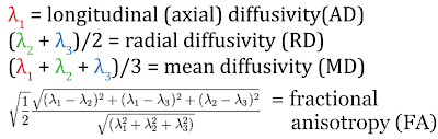
Once that finishes running you can organize the output data, and divide the output values by 10000. This is necessary because to make sure the output values in the weighted mean code have sufficient number of decimals they are multiplied by 10000. Furthermore, this code will also divide trace (TR) values by 3 to get the appropriate value of mean diffusivity (MD = TR/3).

Organize output data:


cd /Volumes/Vol/processed_DTI/weighted_scalars
for scalar in fa tr ad rd;
do
for structure in CING_L CING_R UNC_L UNC_R;
do
rm -f ${structure}_${scalar}_merge.txt;
echo "Subject">>subject${scalar}${structure}.txt;
echo ${structure}_${scalar} >> ${structure}_${scalar}_merge.txt;
for subject in S01 S02 S03 S04;
do
echo ${subject}>>subject${scalar}${structure}.txt;
if [ "${scalar}" == "tr" ]
then
var=`cat *_weighted_output.txt | grep ${subject}|grep ${structure}|grep ${scalar}|awk 'BEGIN{FS=""}{print $4}'`;
value=`bc <<<"scale=8; $var / 30000"`
echo $value >> ${structure}_${scalar}_merge.txt;
else
var=`cat *_weighted_output.txt | grep ${subject}|grep ${structure}|grep ${scalar}|awk 'BEGIN{FS=""}{print $4}'`;
value=`bc <<<"scale=8; $var / 10000"`
echo $value >> ${structure}_${scalar}_merge.txt;
fi
done
mv subject${scalar}${structure}.txt subject.txt;
cat ${structure}_${scalar}_merge.txt;
done
done
#Print data to text file and screen
rm all_weighted_output_organized.txt
paste subject.txt *_merge.txt > all_weighted_output_organized.txt
cat all_weighted_output_organized.txt
This should provide you with a text file with columns for each structure & scalar combination, with rows for each subject. You can then export this to your favorite statistical processing software.
Finally as promised. Code to extract significant cluster from whole brain voxel-wise statistics, in this case from FSL's Randomise output:

Extract binary files for each significant clusters:


#Extract Cluster values for all significant maps
dir=/Volumes/Vol/processed_DTI/
cd $dir;
rm modality_index.txt;
for study in DTI/STUDY_randomise_out DTI/STUDY_randomise_out2;
do
prefix=`echo $study|awk 'BEGIN{FS="randomise_"}{print $2}'`;
cluster -i ${study}_tfce_corrp_tstat1 -t 0.95 -c ${study}_tstat1 --oindex=${study}_cluster_index1;
cluster -i ${study}_tfce_corrp_tstat2 -t 0.95 -c ${study}_tstat2 --oindex=${study}_cluster_index2;
num1=`fslstats ${study}_cluster_index1.nii.gz -R|awk 'BEGIN{FS=""}{print $2}'|awk 'BEGIN{FS="."}{print $1}'`;
num2=`fslstats ${study}_cluster_index2.nii.gz -R|awk 'BEGIN{FS=""}{print $2}'|awk 'BEGIN{FS="."}{print $1}'`
echo $prefix"," $num1 "," $num2;
echo $prefix"," $num1 "," $num2>>modality_index.txt;
#loop through significant clusters
count=1
while [ $count -le $num1 ];
do
fslmaths ${study}_cluster_index1.nii.gz -thr $count -uthr $count -bin /Volumes/Vol/processed_DTI/STRUCTURES/${prefix}_${count}_neg.nii.gz;
let count=count+1
done
count=1
while [ $count -le $num2 ];
do
fslmaths ${study}_cluster_index2.nii.gz -thr $count -uthr $count -bin /Volumes/Vol/processed_DTI/STRUCTURES/${prefix}_${count}_pos.nii.gz;
let count=count+1
done
done

Extract cluster means:


#Extract TFCE cluster means
rm -f *_weighted.nii.gz
rm -f *_weighted_output.txt;
rm -f *_merge.txt;
cd /Volumes/Vol/processed_DTI;
for i in DTI/STUDY_randomise_out DTI/STUDY_randomise_out2;
do
prefix=`echo ${i}|awk 'BEGIN{FS="/"}{print $1}'`;
suffix=`echo ${i}|awk 'BEGIN{FS="/"}{print $2}'`;
rm structures_all.txt;
cd /Volumes/Vol/processed_DTI/STRUCTURES;
for j in `ls ${prefix}_${suffix}*`;
do
pre=`echo ${j}|awk 'BEGIN{FS=".nii"}{print $1}'`;
echo $pre >> /Volumes/Vol/processed_DTI/structures_all.txt;
done
cd /Volumes/Vol5/processed_DTI/NOMOM2/TEMPLATE/normalize_2017;
rm scalars_all.txt;
echo $suffix > scalars_all.txt;
sh ./weighted_mean.sh /Volumes/Vol/processed_DTI/ structures_all.txt scalars_all.txt /Volumes/Vol/processed_DTI/${prefix}/${suffix} S01 S02 S03 S04;
done
Finally, just run the code to organize the output data.

Viewing all 30 articles
Browse latest View live