Visualization tool: 3D Slicer

April 4, 2012, 1:22 pm

≫ Next: DTI Processing - The Basics

$

0

0

3D Slicer is a great visualization program that has a multitude of tools for analysis of medical images, like registration, segmentation, neurosurgical planning and fiber tracking.

The program provides support for DICOM, NRRD, NIFTI, Tiff, JPG, Freesurfer, FITS and a number of other formats. A comprehensive tutorial on diffusion MRI analysis is provided here.  

Download the latest 3D Slicer version here (Windows, Mac OS X and Linux)

More 3D Slicer tutorials

3D Slicer Webinar

---

DTI Processing - The Basics

June 12, 2012, 9:42 am

≫ Next: Reduced Structural Connectivity of a Major Frontolimbic Pathway in Generalized Anxiety Disorder

≪ Previous: Visualization tool: 3D Slicer

$

0

0

Diffusion Tensor Images (DTI) is a cutting edge imaging technique that provides quantitative information with which to visualize and study connectivity of neural pathways. A growing number of studies are now collecting DTI scans which necessitates knowledge in DTI processing steps and tools.

The basic processing pipeline has the following elements:

1. Convert data from scanner to scalar image
2. Run distortion correction

• EPI distortion correction with fieldmap/TOPUP
• Eddy current correction

Brain extraction

Tensor fitting

Produce scalars (FA, MD, AD, RD, RGB)

Advanced processing:

1. Normalization

• Scalar normalization, or
• Tensor normalization

Fiber tracking

• Deterministic, or
• Probabilistic

Whole brain analysis

• Voxel-based analysis, or
• Track-based analysis

The below PDF will give an overview of preprocessing steps like distortion correction and tensor estimation, discuss choices that can be made regarding whole brain versus tract specific analysis, and what normalization and visualization tools are available. Find the presentation here or click the image.

Reduced Structural Connectivity of a Major Frontolimbic Pathway in Generalized Anxiety Disorder

September 5, 2012, 9:22 pm

≫ Next: Video: Corpus Callosum in 3D

≪ Previous: DTI Processing - The Basics

$

0

0

Check out our new study that just got published in Archives of General Psychiatry:

"A new University of Wisconsin-Madison imaging study shows the brains of people with generalized anxiety disorder (GAD) have weaker connections between a brain structure that controls emotional response and the amygdala, the Uncinate Fasciculus, which suggests the brain's "panic button" may stay on due to lack of regulation."

http://archpsyc.jamanetwork.com/article.aspx?articleid=1356405

Here you get an impression of how we traced the Uncinate Fasciculus in all the 88 subjects. You can see a three-dimensional rendering of the Uncinate Fasciculus and the 4 seed areas, overlaid on a Fractional Anisotropy map for a single subject.

http://archpsyc.jamanetwork.com/multimediaPlayer.aspx?mediaid=4197183

Video: Corpus Callosum in 3D

October 5, 2012, 2:38 pm

≫ Next: DTI Processing - Voxel-based versus tract-based diffusion imaging

≪ Previous: Reduced Structural Connectivity of a Major Frontolimbic Pathway in Generalized Anxiety Disorder

$

0

0

This movie shows a colorful 3D rendering of the white matter fiber tracts in the Corpus Callosum (CC), overlaid on a T1 image. Data from the Waisman Laboratory for Brain Imaging and Behavior at University of Wisconsin.

DTI Processing - Voxel-based versus tract-based diffusion imaging

October 21, 2012, 12:38 pm

≫ Next: DTI processing with Camino

≪ Previous: Video: Corpus Callosum in 3D

$

0

0

The
 development
 of
 diffusion
 magnetic resonance imaging (dMRI)

 enabled
 the
 research
 of
 white 
matter 
micro- and macro-structurein 
vivo. 
DMRI 
measures 
the 
magnitude 
and
 orientation
 of 
water
 diffusion.
 This
 is

 done
 in
 multiple
 directions

 to
 calculate
 the
 
 three
 dimensional
 representation
 of
 the
 water
 diffusion
 profile.
  Gray
 matter
 has
 predominantly
 isotropic (soccer ball shaped)
 water
 diffusion, while dense
 white
 matter 
tracks 
have 
highly 
anisotropic 
(rugby ball shaped) diffusion 
of
 water 
pointing 
in 
the
 direction
 of
 the
 fiber
 bundle.


The
 measure
 most 
commonly 
used 
to
 characterize 
directional 
diffusion 
is
 fractional
 anisotropy
 (FA).
 This
 measure
 gives
 a
 value
 between
 0
 and
 1
 to
 indicate
 the
 fraction
 of
 diffusion
 that
 is
 in
 the
 longitudinal
 direction
 compared
 to
 the
 proportion
 of 
diffusion 
in 
both 
transverse
 directions.

 Other measures that can be used are axial diffusivity (AD), radial diffusivity (RD) and mean diffusivity (MD).

Voxel-Based Morphometry

There 
are 
two 
main 
methods 
of 
analyzing diffusion 
images.
 The 
first 
is
 Voxel‐Based
 Morphometry
 (VBM)
 analysis,
 which
 is specifically suited for whole
 brain
 analysis.
 It
 is 
a
 voxel wise 
method 
to
 statistically 
compare 
local 
anisotropy 
values
 for 
the 
whole
 brain 
between 
different 
subjects. It has to be kept in mind that this method should correct for multiple comparisons.
 One way to reduce the number or comparisons is to use an atlas based segmentation methods to selectively investigate white matter areas of interest.

Tract-Based Analysis

The
 second
 method
 is
 called
 tract‐based
 analysis.
 This
 is
 the
 newest
 development
 in
 dMRI
 methodology.
 It
 uses
 the
 more
 anisotropic
 tensors
 to
 form
 streamlines
 of
 tensors
 leading
 to
 estimations
 of
 white
 matter
 fiber
 tracts.
 A
 region
 of
 interest
 is
 used
 as
 seed
 region
 from
 where
 the
 fibers
 are
 traced.
 For
 each
 tract
 mean
 FA
 values
 can be
 calculated.
 These
 values
 per
 tract
 can
 be
 compared
 across
 groups
 to
 investigate
 structural
 connectivity.
 

Voxel
 based
 morphometry
 and
 fiber
 tractography
 are
 two
 methods
 using
 a
 fairly
 different
 approach in dMRI.
 In
 VBM
 the
 whole
 brain
 is
 investigated,
 but
 the
 method
 relies
 heavily
 on
 effective
 registration
 between
 subjects.
 When
 regions
 of
 abnormal
 FA
 values
 do
 not
 map
 onto
 each
 other
 correctly
 this
 will
 greatly
 reduce
 the
 chance to
 find
 significant
 results.
 In
 tract‐based
 analysis
 tracts can be delineated without relying on subject registration. Although specific
 a
 priori
 regions
 of
 interest
 or
 specific
 tracts
 need to be
 selected
 for
 comparison.
 

DTI processing with Camino

November 18, 2012, 7:17 pm

≫ Next: DTI Processing - Tractography tutorial

≪ Previous: DTI Processing - Voxel-based versus tract-based diffusion imaging

$

0

0

UCL has recently added a very comprehensive step-by-step guide to tensor fitting with their Camino software.
From their website:

"This tutorial gives an introduction to standard diffusion tensor image fitting with Camino. It gives a step-by-step guide of how to fit the diffusion tensor to data from DTI or HARDI acquisition protocols, how to generate maps of standard markers like mean diffusivity (MD) and fractional anisotropy (FA), and how to generate principal direction and colour FA maps."

"In steps 1-7, we use a human data set and go through the steps to reconstruct and visualize the tensor information, then we do similar reconstruction on some animal data. There is some overlap between the two examples, but in the animal data we look at additional details, and show how to fix the scheme file so that the orientation of the tensors is correct in the image space."

More information here:

http://cmic.cs.ucl.ac.uk/camino/index.php?n=Tutorials.DTI

DTI Processing - Tractography tutorial

November 18, 2012, 9:04 pm

≫ Next: DTI Scalars (FA, MD, AD, RD) - How do they relate to brain structure?

≪ Previous: DTI processing with Camino

$

0

0

Fiber tractography is a very elegant method that can be used to delineate individual fiber tracts from diffusion images. This tutorial will help you in a step by step way trough the process. 

In the first place you will need to produce both a track file and scalar maps like fractional anisotropy (FA) maps and mean diffusivity (MD) maps. You can either simply download the diffusion toolkit wich is highly compatible with the visualization program TrackVis. Or you can use other tools like the ones from Camino (you will need this camino to trackvis tool) or FSL Diffusion Toolbox. You can find more info on distortion correction and preprocessing here and here.

Once you have done that, the hardest part is pretty much over. Download the tract visualization program TrackVis here. The software is free but you will have to register. TrackVis is compatible with windows, linux and mac. Both the diffusion toolkit and TrackVis are developed by one of the core developers of diffusion imaging; Van Wedeen and Ruopeng Wang. The support for the software is great, questions are readily answered trough their forum and the software is still improving with updates. You will have to keep in mind that this is a three dimensional visualization program so it will demand a fairly decent memory performance depending on the size of your files (voxel size, number of tracts). One hint when running whole brain tractrography is to limit the number of tracts traced by applying a white matter mask (simply cutting off any voxels that have FA values below .15 or .2). Another tip is to use the MD map to get rid of much of the noise rim around the brain - by thresholding out the lowest 10%.

Getting started

Open TrackVis by clicking it in windows and mac, or through the terminal in linux:

> trackvis -new tracts.trk &

The panel on the right of the screen is called the control panel, which includes the overview and property section. The lower panel is called the image panel, which includes three orthogonal brain views, an image section and a ROI section. The main image with the 3D rendering is called the render window.

To load overlay scalar image click this button:

Then choose your scalar file eg.: FA.nii.gz
If you load the scalar but can not see it on the main image play around with Slice Opacity.

Start to draw ROI's: click: 

Choose Hand Draw - click on: 

and:

Play around with the tools

• - What do the other ROI tools do? More on this on the TrackVis website
• - You can only draw ROI's in the image panel and not on the 3D render window. To increase the size of the image panel you can slide it up to make it larger. Double click the render window to hide or show the image panel.
• - You can move the main image in both the render window and image panel by clicking and dragging - you can play around with this
• - Right click the main image to Reset or Straighten
• - Zoom in/out on the orthographic FA images and main image by scrolling - beware this is a slow and sensitive tool.
• - You can move the orthographic FA images with shift and click
• - You can adjust the orthographic FA images brightness with control and click
• - To start selecting specific white matter tracks you can use methods used by:
•   - Mori et al (Imaging Cortical Association Tracts in the Human Brain Using Diffusion-Tensor-Based Axonal Tracking, 2002)
•   - Catani and de Schotten (A diffusion tensor imaging tractography atlas for virtual in vivo dissections, 2008)

How to delineate the Uncinate Fasciculus (UNC)

• - The delineation of the UNC is contingent on finding the correct coronal slice, specifically the most posterior coronal slice that shows clear separation of the frontal and temporal lobes bilaterally. An example is shown in the image below where each of the four UNC ROI's are shown from the image panel:

• - In the right Overview pane in the Objects tab right click Track 1 and select Toggle Existing ROI, choose both left ROI's

• - Then right click Track Groups and click New Track Group From Slice, once that is done toggle the two right ROI's for Track 2
• - In the Property pane expand the options for Slice Filters - Y, for Operator choose Not. Do this for Track 1 and 2.

• - Next you double click Skip and deselect it, do this for both sides.
• - What you see now is roughly all the tracks for the Left and Right Uncinate Fasciculus.

• - The tracks are not perfect yet, we want to get rid of some of the fibers that belong to other pathways or are just wrong

• - Create a new Hand Drawn ROI, choose the rectangle and draw a big rectangle in the middle of the sagittal plane:

• - Toggle this fifth ROI to both Track 1 and 2, and in ROI Filters option for ROI 5 choose Operator - Not.

• - Play around with ROI 5 by adding area's in different planes until you achieve an Uncinate Fasciculus as in the movie below:

• - Now that your Right and Left Uncinate Fasciculi are perfect you can look at the stats, you can find those in the Overview pane underneath the Dataset Info tab. Click on More Stats - View

•  -What is for example the Mean FA of your left Uncinate? And your right? And the whole brain?

• - You can export these thats with Export, do this for each side and the whole brain separately.
• - As a next step it is smart to start saving everything. Start with saving all the ROI's by right clicking them in the Overview pane, then click on Save, try to think of a good naming convention that can include the UNC and the ROI number. 
• - Next click File and Save Scene. The newer versions of trackvis seem to deal with this better but if you run into issues with re-opening your scene file try to save the ROI's before you save the scene or it will not load them correctly once you want to re-open the scene.
• - Now click Track 1 and 2 and save those as NIfTI files, this gives you the option of opening these files in FSLVIEW and see them in 3D:

Now let's play around with some aesthetics:

• - Hide all ROI's
• - Hide the Z-plane by unselecting Z in the orthographic view
• - In the Property pane find Color Code and click on Directional - choose Scalar. By default the FA map will now be used to color code the track, do this for both sides.
• - Adjust the Low and High Threshold for the color coding to be between 0 and 0.5
• - You can also adjust the color spectrum, BUT on certain occasions this will crash the program, so use with care.
• - Also you can choose to Render a tube instead of a line, try this but keep in mind that rendering this will take a moment.
• - The output can then look like this (the overlay in the below images is a T1 image registered to FA):

Final output example

In the image below you can find some of the fiber tracts that are important in autism spectrum disorder (ASD). In green the cingulum, in purple the uncinate fasciculus and in red and blue the arcuate fasciculus and superior longitudinal fasciculus respectively, image from Travers et al. 2012.

DTI Scalars (FA, MD, AD, RD) - How do they relate to brain structure?

January 15, 2013, 3:30 pm

≫ Next: Why Do We Acquire B0 Images in DTI Exams?

≪ Previous: DTI Processing - Tractography tutorial

$

0

0

A key question that is often posed in this field is how neural microstructure relates to the different measures that are extracted from diffusion images (like FA, MD etc). The table below attempts to clarify how differences and changes in biology affect different measures of diffusivity. 

	FA	MD (λ1+λ2+λ3)/3	AD λ1	RD (λ2+λ3)/2
	FA is a summary measure of microstructural integrity. While FA is highly sensitive to microstructural changes, it is less specific to the type of change.	MD is an inverse measure of the membrane density, is very similar for both GM and WM and higher for CSF. MD is sensitive to cellularity, edema, and necrosis.	AD tends to be variable in WM changes and pathology. In axonal injury AD decreases. The ADs of WM tracts have been reported to increase with brain maturation.	RD increases in WM with de- or dys-myelination. Changes in the axonal diameters or density may also influence RD.
Gray Matter	↓	−	↓	↑
White Matter	↑	−	↑	↓
CSF	↓	↑	↑	↑
High myelination	↑	↓	−	↓
Dense axonal packing	↑	↓	−	↓
WM Maturation	↑	↓	↑	↓
Axonal degeneration	↓	↑	↓	↑
Demyelination	↓	↑	−	↑
Low SNR	↓	↑	↓	−

References:

Feldman et al. (2010). Diffusion Tensor Imaging: A Review for Pediatric Researchers and Clinicians. J Dev Behav Pediatr.
Alexander et al.(2012). Characterization of Cerebral White Matter Properties Using Quantitative Magnetic Resonance Imaging Stains. Brain Connectivity.

Definitions:

FA = Fractional Anisotropy
MD = Mean Diffusivity
AD = Axial Diffusivity
RD = Radial Diffusivity
WM = White Matter
GM = Gray Matter
CSF = Cerebral Spinal Fluid
SNR = Signal to Noise Ratio
λ = Eigen Value; length of the axis in the tensor

---

Why Do We Acquire B0 Images in DTI Exams?

February 15, 2013, 7:26 am

≫ Next: Diffusion imaging discussion forum

≪ Previous: DTI Scalars (FA, MD, AD, RD) - How do they relate to brain structure?

$

0

0

This post is in response to the following question that was received from one of our readers:

"I acquired a DTI exam of a patient, which has an artifact that corrupted the B0 images but left the diffusion encoded images unaffected. Can I scan the patient again a year later and use that B0 image to process both exams?"

To answer this question Samuel Hurley was kind enough to write a guest blog post:

                                                                                               

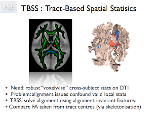
Let us begin by observing the difference between a non-diffusion weighted (left) and diffusion-weighted (right) image:

This image on the left is typically referred to as a "B0 image," although this should not be confused with the variable B0, which describes the the strength of the main magnetic field (e.g. 3T). If we inspect the equation that describes a diffusion weighted imaging (DWI) experiment, we see that the overall level of signal in a DWI image is scaled by a factor S_0:

In addition to acquiring diffusion-weighted data (b>0, right image), we also need to acquire data with b=0:

As we observe from the equation, this gives us an image with signal intensity S_0. We divide each diffusion weighted image S_DWI by this image in order to remove the S_0 scaling term from the equation and properly fit the data to estimate ADC (or the diffusion tensor D, in the case of DTI imaging)
S_0, or the B0 image (as we will refer to it herein), is an image of the anatomy that takes into account tissue signals and contrasts in the absence of diffusion gradients. Because the echo time (TE) is typically long in a DWI or DTI experiment to accommodate large diffusion encoding gradients, this is typically a T2-weighted image. However, in addition to this T2 contrast, there are other factors that modulate the intensity of this image.

One of the main reasons the B0 images are acquired during the same scan as the other DTI encoding directions is due to the scanner's prescan function, which sets the hardware receiver and transmitter gain settings (as well as resonant frequency, shim, and a few other things). These gains determine the way the raw MRI signal in the coil (in volts) is translated into a digitally stored image (as bits and bytes in a file). Each time you run the scan, this gain is re-calibrated, leading to a different signal scale.

DWI and DTI exams are typically acquired with echo-planar imaging (EPI) readouts in order to reduce the overall duration of the experiment as well prevent phase errors induced by the extremely large diffusion encoding gradients. In spite of advances in magnet shimming and parallel imaging (PI), moderate to severe geometric distortion artifacts are still likely in EPI due to field inhomogeneities (e.g. the signal "pileup" in the frontal lobe [left side] of the above images). Removing and re-positioning a patient will alter how that individual's anatomy interacts with the main field, changing the patterns of geometric distortion. While nonlinear coregistration (e.g. FNIRT, ANTs), phase correction algorithms, and eddy current correction (eddy_correct, FSL) can mitigate some of these distortions, they are not effective at completely removing them.

Additionally, the sensitivity profile of the coil also modulates the image intensity, and this profile is likely to be different after the patient has been removed and later re-positioned in the magnet. Coil sensitivities are actually removed using image-based parallel imaging (PI) techniques such as SENSE (ASSET, iPAT), as is typically done with a phased array coil in order to reduce EPI geometric distortion artifacts. However, the SNR (g-factor) and residual PI (aliasing) artifacts in different parts of the image will likely be different. Inconsistent SNR levels between B0 images and diffusion weighted images may bias estimates of ADC or D.
Therefore, the purpose of the B0 images is not only to divide out the baseline T2w signal of tissues, but also to remove these other sources of signal variance listed above.  Receiver gains and voltages tend to drift significantly over the timescale of hours; therefore over the course of a year it is unlikely for these values to remain stable. Additionally, by removing and re-placing the patient's head a year later, the coil sensitivities, geometric distortions, and SNR variations due to PI are no longer likely to match up.

Diffusion imaging discussion forum

March 4, 2013, 11:08 am

≫ Next: DTI Processing - Software Tools

≪ Previous: Why Do We Acquire B0 Images in DTI Exams?

$

0

0

After hosting this diffusion imaging blog for over 4 years I am receiving an increasing amount of questions in my inbox from users. I feel that some of the answers to these questions might benefit more readers and furthermore could benefit from input by other experienced brain imaging researchers. To address this problem I started a diffusion imaging discussion forum. Please feel free to join this group, post questions and add to the discussion. The group is accessible through google, or simply by joining the group and adding your question below.

Note that a google email address in not necessary to sign up. 

DTI Processing - Software Tools

March 26, 2013, 7:16 am

≫ Next: Human Connectome Project

≪ Previous: Diffusion imaging discussion forum

$

0

0

When starting out in a new imaging field like diffusion tensor imaging it is easy to be overwhelmed by different processing steps and tools.

A recent publication from frontiers in neuroscience tries to offer an answer to most of these questions in their appropriately named article: "A hitchhiker's guide to diffusion tensor imaging". You can find the full manuscript here.

The article discusses sources of artifacts during acquisition and how to reduce/correct them, they go into some detail on how to do quality control (expect a post on this topic here soon), what skull stripping methods are available, how you can use RESTORE for robust tensor estimation, etc.

Most importantly, they supply an exhaustive list of DTI software packages that I adapted into the below table.

DTI tools	Pre-processing	Tensor estimation	Fiber tracking	ROI-analysis	Registration
3D Slicer		x	x	x
AFNI	x	x
BioImage Suite		x	x	x
BrainVoyager QX		x	x
Camino		x	x
Dipy		x	x
DoDTI	x	x	x
DTI-Query			x
DTI-TK					x
DTIStudio		x	x	x
ExploreDTI	x	x	x
Freesurfer	x	x
FSL-FDT	x	x	x
FSL-TBSS					x
JIST	x	x
MedINRIA		x	x	x
MrDiffusion		x	x
MRtrix		x	x
SATURN		x	x
SPM (e.g., Diffusion II, DTI)	x	x
TrackVis		x	x	x
TORTOISE	x	x		x
	Pre-processing	Tensor estimation	Fiber tracking	ROI-analysis	Registration

Reference: J.M. Soares, P. Marques, V. Alves, N. Sousa (2013). A hitchhiker's guide to diffusion tensor imaging, Frontiers in Neuroscience.

For my research I use a combination of packages: FSL for preprocessing, Camino for tensor fitting and fiber tracking, DTI-TK for tensor based normalization and TrackVis for visualization and ROI- analysis.

Human Connectome Project

March 28, 2013, 7:29 pm

≫ Next: Share your diffusion imaging news

≪ Previous: DTI Processing - Software Tools

$

0

0

The 40 million dollar human connectome project exemplifies the relevance of studying structural and functional brain connectivity. The NIH awarded this money to a consortium of institutions to provide an unparalleled compilation of neural data, an interface to graphically navigate this data and the opportunity to achieve never before realized conclusions about the living human brain.

The human connectome project will in the near future become an amazing source of publicly available data, so keep an eye on that!

Update:

The Quarter 1 data release with 68 subjects is online! It includes structural, functional (resting state and task) and diffusion images. http://humanconnectome.org/data/

More information:

http://www.humanconnectomeproject.org/
http://www.neuroscienceblueprint.nih.gov/connectome/
http://humanconnectome.org/

Share your diffusion imaging news

May 20, 2013, 2:59 pm

≫ Next: Guest post invitation

≪ Previous: Human Connectome Project

$

0

0

Diffusion-imaging.com would like to know what is new and interesting in DTI research! You can share articles (e.g. your own) on our social media:

https://plus.google.com/+Diffusionimaginggroup

https://www.facebook.com/DiffusionImaging

Guest post invitation

June 3, 2013, 2:19 pm

≫ Next: Diffusion MRI workshop: Videos now online

≪ Previous: Share your diffusion imaging news

$

0

0

Would you like to write a post on a method, study or conference that is diffusion imaging related? Diffusion-imaging.com is now inviting guest writers to contribute to this website.

You can find my contact information here: http://brainimaging.waisman.wisc.edu/~tromp/.

Diffusion MRI workshop: Videos now online

September 11, 2013, 9:15 pm

≫ Next: DTI tutorial for FSL

≪ Previous: Guest post invitation

$

0

0

The videos and slides of the 2013 workshop on diffusion imaging in traumatic brain injury are now available online, with links to the suggested reading materials:

http://tbi.ci.uchicago.edu/diffusion-mri-tbi-workshop

You can find a selection of videos that are of general interest to DTI researchers after the break.

---

DTI-STUDIO software for image processing

Susumu Mori, Johns Hopkins Univ. School of Medicine, Baltimore, Maryland (USA)
Presentation Slides (PDF, PPT)

Further Reading:
DTI Studio

---

CAMINO and DTI-TK advanced diffusion MRI pipeline for traumatic brain injury

Gary Hui Zhang, Univ. College London (UK)
Presentation Slides (PDF, PPT)

Further Reading:
Camino
UCL Microstructure Imaging Group

---

MedInria neuroimaging software system and traumatic brain injury

Oliver Commowick, INRIA VISAGES, Rennes (France)
Presentation Slides (PDF, PPT)

Further Reading:
MedInria

---

DTI tutorial for FSL

September 20, 2013, 4:09 pm

≫ Next: Fibernavigator: Interactive tractography visualization tool

≪ Previous: Diffusion MRI workshop: Videos now online

$

0

0

Check out this website for a great tutorial of diffusion tensor imaging analysis using FSL. It will give you an overview of how to use the FDT Diffusion tool for diffusion imaging analysis, and how you can use MedINRIA (med.inria.fr) to visualize the tracts.

Written by Leigh Morrow, Paul Morgan and Chris Rorden, you can find their site here:

www.cabiatl.com/CABI/resources/dti-analysis/

Additionally check out the lecture on DTI developed by FSL for more information on Tract-Based Spatial Statistics:

fsl.fmrib.ox.ac.uk/fslcourse/lectures/fdt.pdf

Fibernavigator: Interactive tractography visualization tool

October 31, 2013, 12:48 pm

≫ Next: DTI Quality Control - Part 1: Acquisition

≪ Previous: DTI tutorial for FSL

$

0

0

Fibernavigator is an interactive diffusion imaging tractography visualization tool. That, as a bonus, is compatible with DTI data processed by FSL. You can download the open-source software for free from their github website (compatible with windows, mac and linux):

http://scilus.github.io/fibernavigator/

Watch their user tutorial here:

Thanks for the tip Alessandro De Leucio!

DTI Quality Control - Part 1: Acquisition

March 4, 2014, 11:43 am

≫ Next: DTI Quality Control - Part 2: Tensor fitting

≪ Previous: Fibernavigator: Interactive tractography visualization tool

$

0

0

A major issue in DTI image analysis is quality control. Effective quality control for diffusion images relies both on pre tensor fitting (the diffusion weighted images; DWI), and post tensor fitting (the  diffusion tensor images; DTI) checks.

First you will have to check if all volumes were acquired correctly; using fslinfo is one method:

This way you can check if each image has the correct number of volumes and the correct pixel dimensions. Something else you should really pay attention to is the quality of each raw DWI image. If you visually scroll through all the different directions you might come across this:

This does not necessarily have to be a problem if it happens occasionally, but I can become a problem for the tensor calculation if it occurs more frequently (depending on how many directions you acquired).

Next, check the amount of distortion in your image; echo planar imaging (EPI), which is used for diffusion images - are particularly sensitive to stretching in the prefrontal and ventral temporal parts of the brain (depending on the direction of acquisition). For example:

This can be fixed by acquiring a fieldmap that measures the amount of distortion. Read more about this here and here. Or by acquiring data in two opposite directions and then calculating the average. FSL's TOPUP can help out here. 

Some other more serious error images that have no fix:

DTI Quality Control - Part 2: Tensor fitting

March 6, 2014, 8:31 am

≫ Next: DTI Quality Control - Part 3: Tools

≪ Previous: DTI Quality Control - Part 1: Acquisition

$

0

0

After making sure your data was acquired correctly (see also this post) and all looked good - you can go ahead and start tensor fitting. At the core of tensor fitting is using the right gradient directions and sometimes (for programs like Camino) creating a so called "scheme file". A scheme file consists of both the b-values and b-vectors. The b-values are the amount of diffusion weighting used for each volume. Depending on how many non-diffusion weighted or B0 scans you collect (read more on its use here) and what diffusion weighting max you use your b-value file is going to look something like this (shortened version):

0,0,0,0,0,0,1000,1000,1000,1000,1000,1000,1000,1000,1000,1000,1000

Your b-vector are the gradient directions that you collect, often predetermined by the scanner depending on how many total directions you choose to collect. A b-vector file will look something like this (shortened version):

The b-vectors consist out of 3 separate vectors (x, y, z) for each direction acquired. A program like fsl2scheme (more info here) will be able to combine the b-values and b-vectors into a scheme file. Together looking something like this (note that there are 4 b0 slices visible, while the scheme file only shows 1 b0):

If you run a eddy correction it is advisable to correct your scheme file for the induced movement of each volume after registration. Here are a couple of resources to help you with this: 

http://blog.cogneurostats.com/?p=302
http://onlinelibrary.wiley.com/doi/10.1002/mrm.21890/abstract
https://github.com/bernardng/codeSync/blob/master/dMRIanalysis/rotatebvecs
https://www.jiscmail.ac.uk/cgi-bin/webadmin?A2=FSL;3c23f260.0903

After running the tensor fitting command you will have to check if the vectors were applied correctly. In the below examples we are using Camino's pdview, but you can use any program that allows you to view the tensors. You should check the axial, coronal and sagittal views. As a reference the corpus callosum can be used, the tensors should follow the shape of the corpus callosum (in red) in a fluid motion, as in the examples below.

AXIAL VIEW:

CORONAL VIEW:

SAGITTAL VIEW:

EXAMPLE OF WRONG ORIENTATION:

Notice the tensor orientations in corpus callosum (red area)

Fix it by adjusting the scheme file:

There are multiple options to correct the scheme file in the fsl2scheme command:

• add -usegradmod(usually when error pops up)

add -flipx

add -flipy

add -flipz

or any combination of the above, eg. as used in the example above:
fsl2scheme -bvecfile bvecs.txt -bvalfile bvals.txt -flipx -flipy -usegradmod > $prefix.scheme

EXAMPLE OF WRONG COLOR:

Notice the blue corpus callosum

Fix it by adjusting the b-vector table:

• In the bvecs text file, swap the x and z row with the directions.

And in this specific case: fsl2scheme -bvecfile bvecs_zx.txt -bvalfile bvals.txt -flipx -flipz -usegradmod > $prefix.scheme

ANOTHER EXAMPLE:

Notice the green corpus callosum

Fix it by adjusting the b-vector table:

• In the bvecs text file, swap the x and y row.

And in this specific case: fsl2scheme -bvecfile bvecs_yx.txt -bvalfile bvals.txt -usegradmod > $prefix.scheme

Remember:

x - Red
y - Green
z - Blue

DTI Quality Control - Part 3: Tools

March 6, 2014, 8:39 pm

≫ Next: DTI Quality Control - Part 4: Further reading

≪ Previous: DTI Quality Control - Part 2: Tensor fitting

$

0

0

Question:

"We wish to know if there is a quality control program we could run the initial DTI data for each subject through to give us some sort of objective metric output about its quality."  Deborah L. Kerr, Ph.D.

Diffusion imaging quality insurance is very important (as discussed in this and this post) and there are a few - but not nearly enough - tools that can help with that. A fairly new tool is DTIPrep;

DTIPrep is the first comprehensive and fully automatic pre-processing tool for DWI and DTI quality control can provide a crucial piece for robust DTI analysis studies.

It is able to do:

1. Dicom to NRRD converting
2. Image info checking
3. Diffusion information checking
4. Rician LMMSE noise filter
5. Slice-wise intensity checking
6. Interlace-wise intensity checking
7. Averaging baseline images
8. Eddy current and motion correction
9. Gradient-wise checking of residual motion/deformations
10. Joint rician LMMSE noise filter
11. Brain masking
12. DTI computing
13. Dominant direction artifact (vibration artifact) checking
14. Optional visual checking
15. Simulation-based bias analysis

It is unfortunately at this time not yet able to implement a fieldmap correction. Hopefully this will be added soon.
For more information check out their website: http://www.na-mic.org/Wiki/index.php/Projects:DTI_DWI_QualityControl

Or their publication: http://www.ncbi.nlm.nih.gov/pubmed/24523693

Download it here: http://www.nitrc.org/projects/dtiprep/

A different toolbox, called Camino, helps you estimate the signal to noise ratio (SNR) and noise variance of your diffusion image. The tool is called estimatesnr. Their explanation is somewhat complicated but what it comes down to is this -
If you have 2 B0 images: 

The traditional method for estimating the noise is to sample two ROIs, one in brain white matter, and one in the background. Assuming that the background signal contained only noise, we can estimate the noise standard deviation as

  sigma = sqrt(2.0 / (4.0 - PI)) * stddev(signal in background region)

where the constant scaling corrects for the Rician distribution of the noise, giving us the standard deviation sigma of the original signal. To synthesize data with the same noise conditions, we would take the true signal S_0 and calculate

  S = |[S_0 + N(0, sigma), N(0, sigma)]|

where N(0, sigma) is a random sample drawn from normal distribution with mean 0 and standard deviation sigma.

If you have more than 2 B0 images:

The second method requires multiple b=0 images, and defines sigma_mult as the standard deviation of the signal over the ROI, across all K b=0 images. Again, let i be a voxel index, then

  sigma_i = stddev(S_{i1},...,S{iK}))  sigma_mult = mean(sigma_1,...,sigma_N)

And finally SNR is

  mean(S_{11}, S_{12},...,S_{1K}, S_{21},...,S_{NK}) / sigma_mult

If there are two or more b=0 images, both snr_diff and snr_mult will both be computed. The more b=0 images there are, the better the estimate via sigma_mult, but sigma_diff only ever uses the first two b=0 images.

You can use a combination of SNR and maximum intensity of the DWI image - as extracted with fslstats option -r - to get insight into the quality of the data: